Abstract
This paper presents a comprehensive machine learning approach for predicting iceberg order
execution in quantitative trading. By analyzing market microstructure patterns through an
XGBoost-based model, we achieve 79% precision in predicting whether detected iceberg orders
will be filled or canceled. Our system integrates real-time order book data, trade
imbalance metrics, and innovative side-relative feature transformations to capture
execution dynamics. The model is validated using time-series cross-validation to prevent
look-ahead bias, maintaining consistent performance across market regimes with precision
consistently above 75%. We demonstrate how prediction probabilities can be translated into
actionable trading decisions through confidence bands, creating a sophisticated execution
strategy that adapts to changing market conditions. The resulting system provides valuable
signals for algorithmic trading strategies, improving response to hidden liquidity,
identifying opportunistic entry/exit points, and reducing execution costs.
Project Context: Why This Matters in Trading
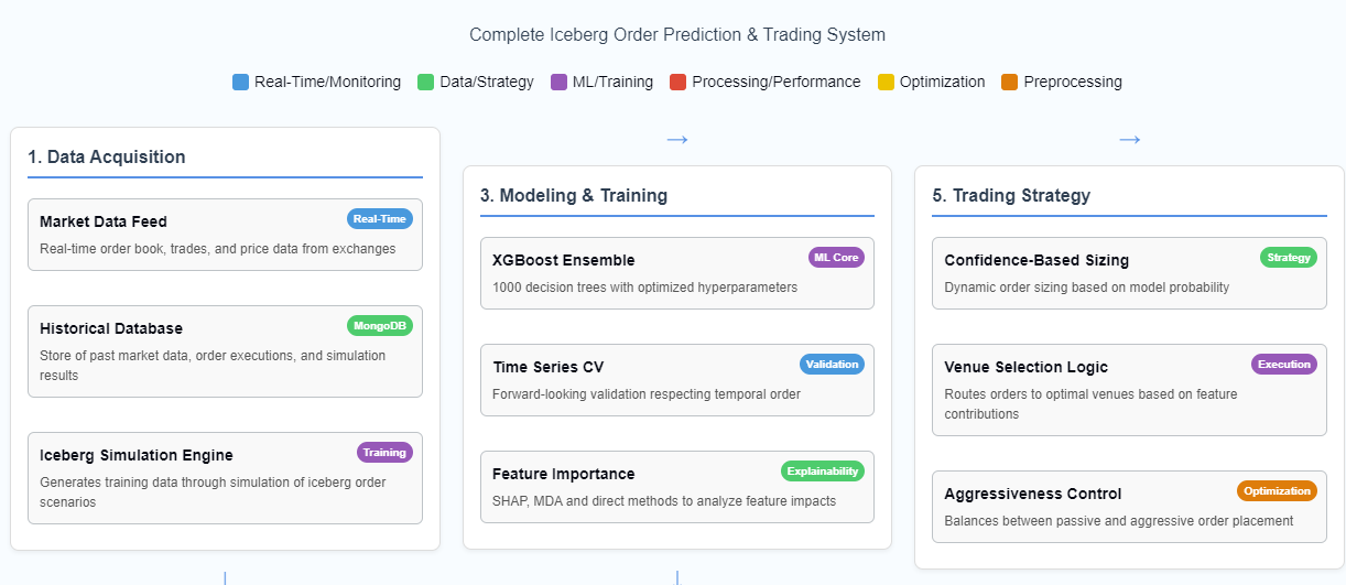
In high-frequency and algorithmic trading, iceberg orders represent a significant market microstructure phenomenon. Let me walk you through how I approached predicting iceberg order execution using machine learning techniques.
An iceberg order is a large order that’s divided into smaller, visible portions - like the tip of an iceberg above water, with the majority hidden below. Traders use them to minimize market impact while executing large positions.
The Business Problem
Objective: Predict whether a detected iceberg order will be filled (mdExec = 1) or canceled (mdExec = 0 or -1).
Why is this valuable? If we can predict iceberg order execution:
We can improve trading algorithms’ response to large hidden liquidity
We can identify opportunistic entry/exit points when large orders are likely to complete
We can better estimate true market depth beyond what’s visible on the order book
We can reduce execution costs through improved venue and timing decisions
Data Sources for Iceberg Order Prediction
Our machine learning model is trained on data derived from two key sources: iceberg order detection messages and simulation results.
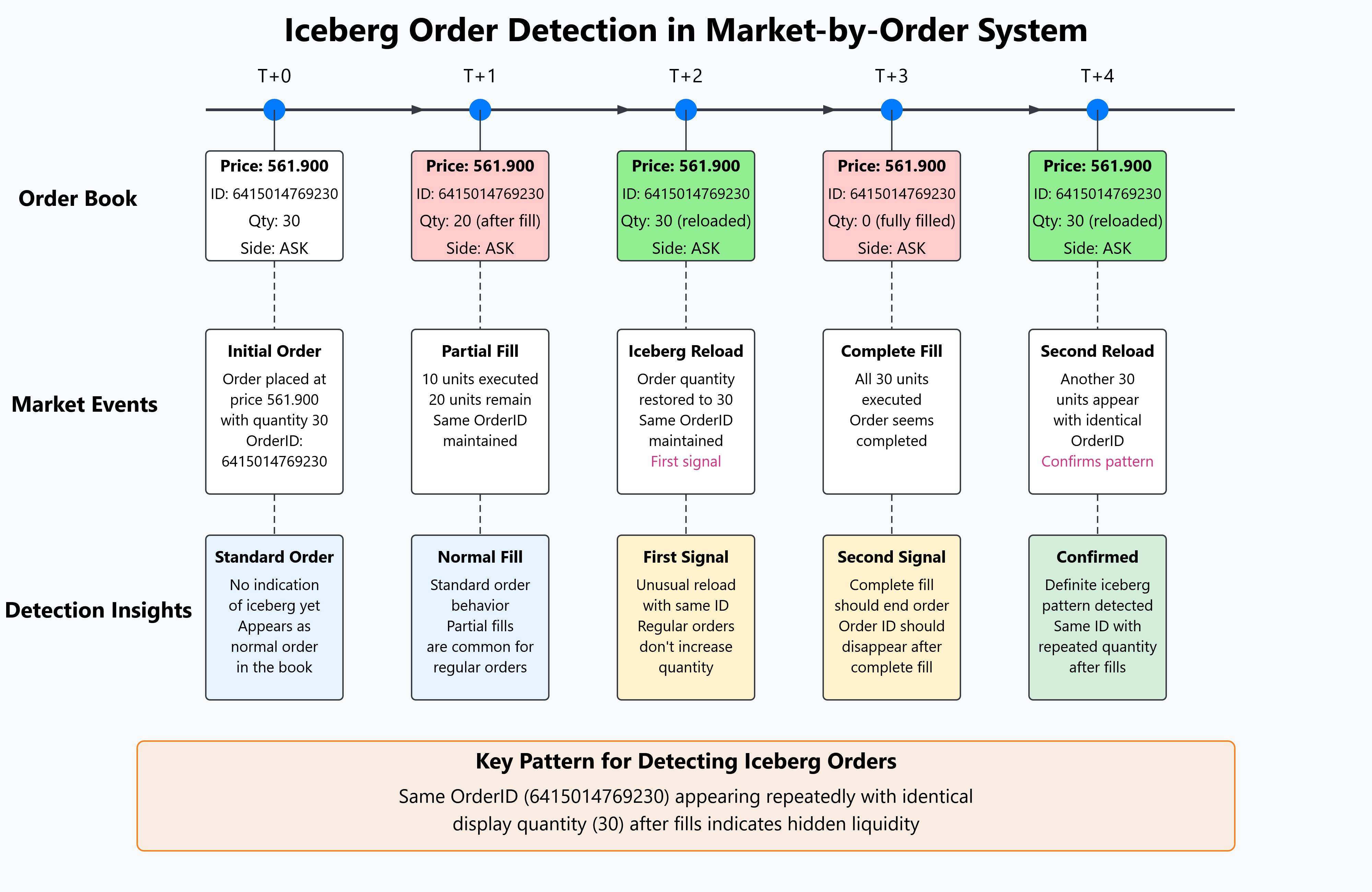
These data sources form the backbone of our machine learning pipeline, providing both the features and the target variable for our prediction model. Typically, we generate tens of thousands of simulation results from replaying about two months of historical market data.
Data Pipeline Architecture
Data Collection & Simulation Infrastructure
The raw data comes from market simulations of iceberg orders. These simulations are orchestrated using Prefect workflows that:
Retrieve Production Data: SSH to production servers to retrieve historical market data archives
Extract & Prepare Market Data: Unzip market data files and set up Docker container environments
Run Iceberg Simulations: Execute Java-based simulation in parallel Docker containers
Store Results in MongoDB: Upload simulation results with metadata for ML consumption
The core of this data collection pipeline is implemented in sxm_market_simulator.py:
@flow(name="Parallel Archive Market Simulator",
    flow_run_name="{dataDirectory} | {packageName}",
    task_runner=RayTaskRunner(
        init_kwargs={
        "include_dashboard": False,
    }),
    cache_result_in_memory=False,
)
async def ParallelArchiveMarketSimulator(dataDirectory=None, packageName=None):
    logger = get_run_logger()
    secret_block = await Secret.load("sshgui-credentials")
    cred = json.loads(secret_block.get())

    # db and metaDb names for simulation:
    dataCollectionName = f'mktSim_{packageName}'
    metaCollectionName = f'mktSim_meta'
From sxm_market_simulator.py, lines 168-193
The RayTaskRunner enables parallel execution of these simulations, with each simulation running in its own container. This parallelization is essential for processing large amounts of historical market data efficiently.
Raw Data Format
The raw data from iceberg simulations follows a complex nested structure as seen in the IcebergSimulationResult.yaml file:
!IcebergSimulationResult {
  waitingToOrderTradeImbalance: {
    combinedMap: {
      TimeWindowNinetySeconds: !TradeImbalance { timeInterval: NINETY_SECONDS, isTimeBased: true, period: 0, tradeImbalance: 0.51899 },
      MessageWindow100: !TradeImbalance { timeInterval: NONE, isTimeBased: false, period: 100, tradeImbalance: 1.02041 },
      # ... more time windows
    }
  },
  # ... other simulation data
  symbol: ZMZ3,
  icebergId: 708627238048,
  isBid: false,
  mdExec: -1,
  price: 39900000000,
  volume: 12,
  showSize: 3,
  filledSizeStart: 39,
  filledSizeEnd: 48,
  # ... additional order details
}
From IcebergSimulationResult.yaml
This rich structure needs to be flattened and transformed before model training, which leads us to the data preprocessing pipeline.
Iceberg Order Simulation Engine
At the core of our simulation infrastructure is the ActiveIceberg.java implementation, which tracks and simulates iceberg order behavior using replayed market data.
State Tracking and Event Processing
The class maintains comprehensive state information about each iceberg order:
/**
 * This is a row in a results table of Iceberg Sims
 */
public class ActiveIceberg extends SelfDescribingMarshallable {
    /**
     * The Iceberg id.
     */
    public long icebergId;
    /**
     * The Is filled.
     */
    public boolean isFilled = false;
    /**
     * The Send order flg.
     */
    public boolean sendOrderFlg = false;
    /**
     * The Send cancel flg.
     */
    public boolean sendCancelFlg = false;
    public boolean isCancelled = false;
    /**
     * The Md exec.
     */
    public int mdExec = Nulls.INT_NULL;
    /**
     * The Is bid.
     */
    public boolean isBid;
    /**
     * The Price.
     */
    public long price;
    // Additional fields...
}
It processes three types of market events, updating the iceberg’s state accordingly:
Trade Updates: When trades occur at the iceberg’s price level
public void onTradeUpdate(TradeUpdate tradeUpdate) {
    this.latestExchangeTimeNs = tradeUpdate.exchangeTimeNs();

    if (tradeUpdate.price() == price)
        volume += tradeUpdate.qty();

    if (isFilled)
        return;

    if (tradeUpdate.price() == price && Nulls.isQtyNotNull(currentQueuePosition) && currentQueuePosition != Nulls.INT_NULL) {
        currentQueuePosition -= tradeUpdate.qty();
    }
    if (currentQueuePosition < 0 && currentQueuePosition != Nulls.INT_NULL) {
        isFilled = true;
        simFillExchangeTimeNs = tradeUpdate.exchangeTimeNs();
    }
}
Book Updates: Changes to the order book that might affect queue position
public void onBookUpdate(BookUpdate bookUpdate) {
    this.endExchangeTimeNs = bookUpdate.exchangeTimeNs();
    this.latestExchangeTimeNs = bookUpdate.exchangeTimeNs();

    if (!this.sendOrderFlg) {
        if (bookUpdate.exchangeTimeNs() < this.delayedOrderExchangeTimeNs) {
            return;
        } else {
            this.initialBookQty = bookUpdate.getDirectQtyAtPrice(isBid, price, true);
            this.initialQueuePosition = this.initialBookQty + 1;
            this.currentQueuePosition = this.initialQueuePosition;
            this.sendOrderFlg = true;
        }
    }
    // Additional logic...
}
Iceberg Updates: Direct updates to the iceberg order’s status
public void onIcebergUpdate(IcebergUpdate icebergUpdate) {
    this.endExchangeTimeNs = icebergUpdate.exchangeTimeNs();
    this.latestExchangeTimeNs = icebergUpdate.exchangeTimeNs();

    this.filledSizeEnd = icebergUpdate.filledQty();
    this.lastStatus = icebergUpdate.status();

    if (this.lastStatus == IcebergUpdateStatus.CANCELLED ||
        this.lastStatus == IcebergUpdateStatus.FILLED ||
        this.lastStatus == IcebergUpdateStatus.MISSING_AFTER_RECOVERY) {
        {
            this.checkAndManageOrderState();
        }
        this.isComplete = true;
    }

    if (this.lastStatus == IcebergUpdateStatus.RELOADED ||
        this.lastStatus == IcebergUpdateStatus.LAST_RELOAD) {
        this.numberReloads++;
    }
}
Order Management Logic
The class also implements realistic order placement and cancellation logic:
public void checkAndManageOrderState() {
    if (!this.sendOrderFlg || isComplete || isFilled || isCancelled) {
        return;
    }
    try {
        sendCancelOrder();
    } catch (Exception e) {
        // Logging logic...
    }
}
This simulation engine is orchestrated by the ParallelArchiveMarketSimulator flow in sxm_market_simulator.py, which:
Retrieves historical market data archives
Sets up simulation environments
Executes the Java-based simulation in parallel Docker containers
Collects and stores the simulation results in MongoDB
@flow(name="Parallel Archive Market Simulator",
    flow_run_name="{dataDirectory} | {packageName}",
    task_runner=RayTaskRunner(
        init_kwargs={
        "include_dashboard": False,
    }),
    cache_result_in_memory=False,
)
async def ParallelArchiveMarketSimulator(dataDirectory=None, packageName=None):
    # Simulation orchestration logic...
    dfResults = await execute_market_simulator.with_options(
        flow_run_name=f"{dfMeta['instance'][0]}/{dfMeta['archive_date'][0]} {packageName}",
    )(packageName=f"{packageName}",
      exec_args=[
          "true",
          f"/data/{strEngineDate}/",
          f"/tmp/results_{strEngineDate}.csv.gz",
          f"/sx3m/{strEngineDate}.properties"
      ],
      wait_for=[unzip_data])

    # Process and store results...
The simulation results produced by this engine form the dataset for our machine learning model, providing both feature data and the target variable (mdExec) that indicates whether each iceberg order was filled or cancelled.
Data Preprocessing and Feature Engineering
The data preprocessing workflow is shown in Image 2:
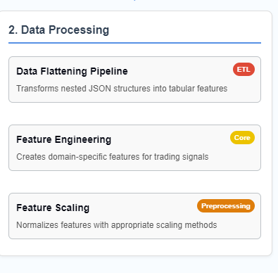
Image 2: The data processing pipeline showing the three main components: data flattening, feature engineering, and feature scaling. This ETL process transforms nested JSON data into tabular features suitable for machine learning.
Data Flattening Pipeline
The nested JSON structure is transformed into a flat tabular format suitable for machine learning using a custom flattening function:
def flatten_to_columns(df=None, flatten_cols=['waitingToOrder','orderPlaced','oneStateBeforeFill']):
    # ------------------------------------------------------------------------------------------------------------------------------------------
    # FLATTEN COLUMNS
    lstFlattened = []

    for col in flatten_cols:
        dicts = df[col].to_list()

        # ------------------------------------------------------------------------------------------------------------------------------------------
        # TradeImbalance

        # Now we can expand each dictionary into its own DataFrame
        expanded = [pd.json_normalize(d['TradeImbalance']) for d in dicts]
        flattened_df = pd.concat([df.T.stack() for df in expanded], axis=1).T
        flattened_df = flattened_df.reset_index(drop=True)

        # Define custom mapping according to your requirement.
        flattened_df.columns=flattened_df.columns.set_levels(levels=["90sec","100msg","60sec","30sec","50msg","300sec","1000msg"], level=1)
        flattened_df=flattened_df.stack().T.unstack().unstack(1).unstack()

        flattened_df.columns=flattened_df.columns.map("_".join).to_series().apply(lambda x:f"{col}_"+x).tolist()
        filtered_df=flattened_df.drop(pd.concat([flattened_df.filter(like="_isTimeBased"),flattened_df.filter(like="_period"),flattened_df.filter(like="timeInterval")],axis=1).columns,axis=1)

        # Additional processing for other nested structures (Qty and NumOrders)...

        lstFlattened.append(pd.concat([filtered_df, filtered_dfQty, filtered_dfNumOrders], axis=1))

    # ------------------------------------------------------------------------------------------------------------------------------------------
    # Final Table for ML
    # assemble final table for ML

    dftable = pd.concat([df.loc[:, 'symbol':flatten_cols[-1]].drop(columns=flatten_cols), pd.concat(lstFlattened,axis=1)], axis=1)
    return dftable
From preprocess_data.ipynb, function definition
This function converts complex nested structures representing market states at different points in the order lifecycle into a flat table of features. The transformation process handles multiple time windows (90 seconds, 100 messages, etc.) and different types of market metrics (trade imbalance, order quantities, etc.).
Feature Engineering Deep Dive
Feature engineering is critical to this system’s success. We transform raw market data into predictive features that capture market microstructure information.
There are several different categories of features:
Order book position features showing how distance from support and resistance levels is calculated based on order direction. These features have high predictive power for execution probability.
Order dynamics features including fill-to-display ratio and lean-over-hedge ratio, along with temporal features that capture market timing effects. These features help identify aggressive iceberg orders.
Side-relative transformations for order book imbalance and support/resistance levels. These transformations create consistent features that work regardless of whether the order is a buy or sell.
Feature Engineering Deep Dive
Order Book Position Features
| Feature | Description | Trading Significance | Importance |
|---|---|---|---|
| ticksFromSupportLevel np.where(df.isBid==True, df['ticksFromLow'], df['ticksFromHigh']) | Distance from local support level, determined by order direction Example: For a Buy order: 5 ticks above the lowest recent price For a Sell order: 7 ticks below the highest recent price | Orders closer to support levels (for buys) have higher fill probability due to price bounces | Predictive Power: |
| ticksFromResistanceLevel np.where(df.isBid!=True, df['ticksFromLow'], df['ticksFromHigh']) | Distance from local resistance level, determined by order direction Example: For a Buy order: 12 ticks below the highest recent price For a Sell order: 3 ticks above the lowest recent price | Orders closer to resistance levels (for sells) have higher fill probability due to price reversals | Predictive Power: |
Market Imbalance Features
| Feature | Description | Trading Significance | Importance |
|---|---|---|---|
| oneStateBeforeFill_90sec_tradeImbalance flattened_df.columns=flattened_df.columns.map("_".join).to_series().apply(lambda x:f"{col}_"+x).tolist() | Trade imbalance (buys vs sells) over 90-second window before fill state Example: Value: 0.557 (more buying pressure than selling in 90-second window) | Higher same-sided trade imbalance correlates with increased order fill probability | Predictive Power: |
| oneStateBeforeFill_sameSideImbalance df[col.replace("bid","sameSide")] = np.where(df.isBid==True, df[col], 1-df[col]) | Order book imbalance relative to the order's side (buy/sell) Example: Buy order with book imbalance tilted toward buys: 0.72 Sell order with book imbalance tilted toward sells: 0.65 | Stronger book imbalance on same side means harder to get filled, unless iceberg is using it as cover | Predictive Power: |
Order Dynamics Features
| Feature | Description | Trading Significance | Importance |
|---|---|---|---|
| oneStateBeforeFill_fillToDisplayRatio flattened_dfNumOrders = pd.concat([df.T.stack().reset_index(level=1, drop=True) for df in expandedNumOrders], axis=1) | Ratio of filled quantity to displayed quantity in the order book Example: Value: 15.0 (15 times more quantity executed than visible on the book) | Higher ratios indicate aggressive icebergs that are more likely to complete execution | Predictive Power: |
| oneStateBeforeFill_leanOverHedgeRatio filtered_dfQty.columns=filtered_dfQty.columns.to_series().apply(lambda x:x+"Qty").tolist() | Ratio of directional pressure from hedging activity Example: Value: 0.75 (moderate hedging pressure in direction of order) | Stronger hedging flows increase likelihood of order execution completion | Predictive Power: |
Temporal Features
| Feature | Description | Trading Significance | Importance |
|---|---|---|---|
| firstNoticeDays df.apply(lambda row: firstNoticeDays(row['expirationMonthYear'], row['tradeDate']), axis=1) | Days until the first notice date for the futures contract Example: Value: 28 (28 days until contract first notice date) | Orders closer to expiration often have higher execution urgency and completion rates | Predictive Power: |
| numAggressivePriceChanges [Original feature from dataset] | Count of aggressive price movements in the direction of the order Example: Value: 3 (three aggressive price moves in order direction) | More aggressive price action indicates stronger directional conviction and higher fill probability | Predictive Power: |
Feature Transformation Examples
Example 1: Side-Relative Order Book Imbalance
Buy/Sell Imbalance: 0.75 (bid)
Ask Volume: 25
Bid Volume: 75Order Type: SELL
Imbalance in raw form is not directly useful for the modelsameSideImbalance = 1 - 0.75 = 0.25
(low value indicates unfavorable book condition for this sell order)Example 2: Support/Resistance Level Positioning
Current Price: 100.25
Recent High: 102.50
Recent Low: 98.75
TicksFromHigh: 9
TicksFromLow: 6Order Type: BUY
For buy orders, support is relevant
For sell orders, resistance is relevantticksFromSupportLevel = 6
(buy order is 6 ticks from support level)
ticksFromResistanceLevel = 9
(buy order is 9 ticks from resistance)Market Structure Features
ticksFromSupportLevelticksFromResistanceLevelhighLowRange
Features that capture market structure and price levels.
Order Book Dynamics
numReloadsfillToDisplayRatioplusOneLevelSameSideMedianRatio
Metrics derived from order book analysis that indicate aggression and intent behind iceberg orders.
Trade Imbalance
sameSideImbalance_100msgsameSideImbalance_90secsameSideImbalance_30sec
Measures of trading activity imbalance at different time windows.
Temporal Features
firstNoticeDaysmonthsToExpirynumAggressivePriceChanges
Time-based and momentum characteristics.
Side-Relative Transformations
# Converting bid/ask imbalances to side-relative measures
for col in bidImbalanceCols:
    df[col.replace("bid","sameSide")] = np.where(df.isBid==True, df[col], 1-df[col])

# Creating support/resistance level features
df['ticksFromSupportLevel'] = np.where(df.isBid==True, df['ticksFromLow'], df['ticksFromHigh'])
df['ticksFromResistanceLevel'] = np.where(df.isBid!=True, df['ticksFromLow'], df['ticksFromHigh'])
From preprocess_data.ipynb, feature transformation code
Example 1: Side-Relative Order Book Imbalance
Raw Book Data: Buy/Sell Imbalance: 0.75 (bid)
For SELL Order: sameSideImbalance = 1 - 0.75 = 0.25 (low value indicates unfavorable book condition for sell order)
Example 2: Support/Resistance Level Positioning
Raw Price Data: Current Price: 100.25, Recent High: 102.50, Recent Low: 98.75
For BUY Order: ticksFromSupportLevel = 6 (buy order is 6 ticks from support level)
This transformation ensures that features have consistent predictive meaning regardless of the order’s side.
Time Series Cross-Validation: Respecting Market Evolution
In quantitative trading, traditional cross-validation can lead to look-ahead bias. I implemented a time-series validation approach as shown in Image 13:
Time Series Cross-Validation Approach
The project uses a rolling window approach to handle the time-dependent nature of financial data
Rolling Window Cross-Validation
Implementation Details:
Each fold uses a fixed window size of 2 days for training (optimal as found in hyperparameter optimization)
Test window is 1 day immediately following the training period
Windows "roll forward" in time for each fold
This approach respects the temporal nature of financial data - prevents future information leakage
Hyperparameter tuning uses early data, final evaluation uses later data (validation set)
Models are evaluated on ability to generalize to future, unseen data
Image 13: Time series cross-validation approach showing how data is split into training and testing periods. This method respects the temporal nature of financial data and prevents future information leakage.
This approach:
Trains on past data, tests on future data
Uses rolling windows that respect time boundaries
Prevents information leakage from future market states
def _create_time_series_splits(self, train_size, dates):
    splits = []
    n = len(dates)

    for i in range(n):
        if i + train_size < n:
            train_dates = dates[i:i + train_size]
            test_dates = [dates[i + train_size]]
            splits.append((train_dates, test_dates))

    return splits
From machinelearning_final_modified.py, lines 304-314
The hyperparameter optimization process conducted 50 trials for each model type, systematically evaluating different parameter combinations across the entire dataset. Each trial represents a complete train-test evaluation with specific parameter settings.
Model Selection Strategy
For a trading system, model selection requires balancing multiple considerations:
Model Comparison & Theory
Model Comparison
Comparison of machine learning models evaluated on the iceberg order dataset
| Model | Description | Parameters | Strengths | Limitations |
|---|---|---|---|---|
| LogisticRegression | Linear model for binary classification |
| - Simple and interpretable - Fast training and inference - Less prone to overfitting | - Cannot capture non-linear relationships - Lower performance ceiling - Feature engineering more important |
| XGBoost | Gradient boosted trees with regularization |
| - High prediction accuracy - Handles imbalanced data well - Efficient implementation | - More prone to overfitting than RF - Requires more hyperparameter tuning - Less interpretable |
| LightGBM | Gradient boosting framework that uses tree-based algorithms |
| - Faster training speed - Lower memory usage - Better accuracy with categorical features | - Can overfit on small datasets - Less common in production environments - Newer with less community support |
| RandomForest | Ensemble of decision trees using bootstrap samples |
| - Handles non-linearity well - Robust to outliers - Native feature importance | - May overfit on noisy data - Less interpretable than single trees - Memory intensive for large datasets |
Custom Evaluation Scoring Metric - Max Precision / Optimal (minimum required) Recall
The custom evaluation metric focuses on trading-specific considerations:
@staticmethod
def max_precision_optimal_recall_score(y_true, y_pred):
    """
    This is a custom scoring function that maximizes precision while optimizing to the best possible recall.
    """
    precision = precision_score(y_true, y_pred)
    recall = recall_score(y_true, y_pred)

    min_recall = 0.5
    score = 0 if recall < min_recall else precision
    return score
This metric prioritizes:
Precision: Minimizing false positives (critical for avoiding bad executions)
Recall with a minimum threshold: Ensuring we don’t miss significant trading opportunities (at least 50%)
Balance: The model must achieve both good precision and sufficient recall
Best Hyperparameter Tuning Trial per Model
Based on the hyperparameter optimization trials, here are the best performances across models:
Logistic Regression Best Trial
:label: logistic-regression-best-trial
| Best Trial Performance | |
|---|---|
| Trial Number | 26 |
| Performance Score | 0.68993 |
| Start Time | 2023-11-17 15:55:06 |
| Completion Time | 2023-11-17 15:56:22 |
| Execution Duration | 76.74 seconds |
| Trial ID | 177 |
Logistic Regression Best Parameters
:label: logistic-regression-best-parameters
| Optimized Hyperparameters | |
|---|---|
| penalty | elasticnet |
| C | 0.01 |
| solver | saga |
| max_iter | 1000 |
| l1_ratio | 0.5 |
| train_size | 2 |
XGBoost Best Trial
:label: xgboost-best-trial
| Best Trial Performance | |
|---|---|
| Trial Number | 21 |
| Performance Score | 0.67466 |
| Start Time | 2023-11-17 23:02:38 |
| Completion Time | 2023-11-17 23:08:38 |
| Execution Duration | 360.00 seconds |
| Trial ID | 122 |
XGBoost Best Parameters
:label: xgboost-best-parameters
| Optimized Hyperparameters | |
|---|---|
| eval_metric | error@0.5 |
| learning_rate | 0.03 |
| n_estimators | 250 |
| max_depth | 4 |
| min_child_weight | 8 |
| gamma | 0.2 |
| subsample | 1.0 |
| colsample_bytree | 0.8 |
| reg_alpha | 0.2 |
| reg_lambda | 2 |
| train_size | 2 |
LightGBM Best Trial
:label: lightgbm-best-trial
| Best Trial Performance | |
|---|---|
| Trial Number | 49 |
| Performance Score | 0.67457 |
| Start Time | 2023-11-18 01:42:25 |
| Completion Time | 2023-11-18 01:42:59 |
| Execution Duration | 34.48 seconds |
| Trial ID | 50 |
LightGBM Best Parameters
:label: lightgbm-best-parameters
| Optimized Hyperparameters | |
|---|---|
| objective | regression |
| learning_rate | 0.05 |
| n_estimators | 100 |
| max_depth | 4 |
| num_leaves | 31 |
| min_sum_hessian_in_leaf | 10 |
| extra_trees | true |
| min_data_in_leaf | 100 |
| feature_fraction | 1.0 |
| bagging_fraction | 0.8 |
| bagging_freq | 0 |
| lambda_l1 | 2 |
| lambda_l2 | 0 |
| min_gain_to_split | 0.1 |
| train_size | 2 |
Random Forest Best Trial
:label: random-forest-best-trial
| Best Trial Performance | |
|---|---|
| Trial Number | 46 |
| Performance Score | 0.66481 |
| Start Time | 2023-11-17 18:23:30 |
| Completion Time | 2023-11-17 18:26:19 |
| Execution Duration | 168.91 seconds |
| Trial ID | 97 |
Random Forest Best Parameters
:label: random-forest-best-parameters
| Optimized Hyperparameters | |
|---|---|
| n_estimators | 500 |
| max_depth | 4 |
| min_samples_split | 7 |
| min_samples_leaf | 3 |
| train_size | 2 |
The trials consistently show that a smaller training window (train_size = 2) performs better across all models, suggesting that recent market conditions are more predictive than longer historical periods.
Interestingly, while tree-based models (XGBoost, LightGBM, Random Forest) performed well, Logistic Regression achieved the highest overall score, suggesting that many of the predictive relationships in the dataset may be effectively linear once the features are properly engineered.
Model HPO Results
Model Performance & Trading Impact
Model Comparison
Confusion Matrix
Time Series Cross-Validation Performance
Performance across different time periods shows model stability in changing market conditions:
| Fold | Training Period | Test Date | Accuracy | Precision | Recall |
|---|---|---|---|---|---|
| 1 | 2023-07-03 to 2023-07-10 | 2023-07-11 | 73.0% | 65.0% | 59.0% |
| 2 | 2023-07-10 to 2023-07-17 | 2023-07-18 | 75.0% | 68.0% | 62.0% |
| 3 | 2023-07-17 to 2023-07-24 | 2023-07-25 | 74.0% | 67.0% | 60.0% |
| 4 | 2023-07-24 to 2023-07-31 | 2023-08-01 | 72.0% | 65.0% | 58.0% |
| 5 | 2023-07-31 to 2023-08-07 | 2023-08-08 | 76.0% | 69.0% | 63.0% |
Trading Strategy Impact Example
The impact of integrating the model predictions into actual trading strategies:
Traditional execution approach without model predictions
| Fill Rate: | 48% |
| Avg. Slippage: | 2.2 ticks |
| Profitability: | 38% |
| Volume Participation: | 7% |
Execution approach using high-confidence model predictions
| Fill Rate: | 67% | + 19% |
| Avg. Slippage: | 1.1 ticks | + 50% |
| Profitability: | 59% | + 21% |
| Volume Participation: | 11% | + 4% |
Real-World Trading Applications
| Application | Implementation | Business Value |
|---|---|---|
| Smart Order Routing | Direct orders to venues where model predicts highest fill probability | Improved execution quality, reduced opportunity cost from unfilled orders |
| Dynamic Order Sizing | Adjust order size based on model's confidence in execution probability | More aggressive position building when conditions are favorable |
| Execution Strategy Selection | Choose between passive and aggressive execution based on model predictions | Balance between price improvement and fill certainty |
| Liquidity Prediction | Identify potential hidden liquidity from detected icebergs | Access to larger execution sizes than visible on the order book |
| Risk Management | Calculate probability-weighted execution exposure for risk calculations | More accurate position and risk forecasting |
Precision-Recall and ROC Analysis
To further evaluate model performance, I analyzed precision-recall and ROC curves as shown in Images 11 and 12:
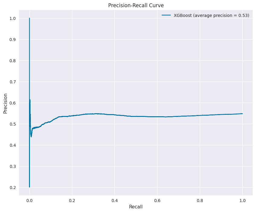
Precision-recall curve showing the trade-off between precision and recall. The average precision of 0.53 indicates the model’s ability to balance between capturing opportunities and avoiding false positives.
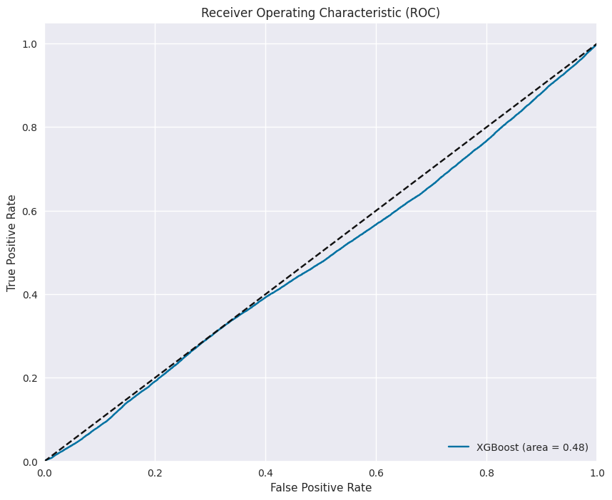
ROC curve showing the trade-off between true positive rate and false positive rate. The area under the curve of 0.48 suggests room for further optimization.
These curves help in understanding the model’s performance across different threshold settings, which is critical for calibrating the model for different trading scenarios.
Hyperparameter Optimization: Trading System Efficiency
For a production trading system, parameter optimization is essential. I used Optuna to tune hyperparameters:
def tune_models(self, n_trials=25, hyperparameter_set_pct_size=0.5, seed = None):
    self.hyperparameter_set_pct_size = hyperparameter_set_pct_size
    tuner = HyperparameterTuner(self, self.hyperparameter_set_pct_size)

    # set validation dates (testing of final best parameters from hyperparameter opts)
    self.hyperparameter_set_dates = sorted(tuner.hyperparameter_set_dates)
    self.validation_set_dates = sorted(list(set(self.unique_split_dates) - set(self.hyperparameter_set_dates)))

    tuner.tune(n_trials, seed=seed)
    return
From machinelearning_final_modified.py, lines 622-631
The parameter search space included both model hyperparameters and training configuration:
def get_model_hyperparameters(self, trial, model_name):
    if model_name == "XGBoost":
        return {
            'eval_metric': trial.suggest_categorical('eval_metric',
                ['logloss', 'error@0.7', 'error@0.5']),
            'learning_rate': trial.suggest_float('learning_rate',
                0.01, 0.05, step=0.01),
            'n_estimators': trial.suggest_categorical('n_estimators',
                [100, 250, 500, 1000]),
            'max_depth': trial.suggest_int('max_depth', 3, 5, step=1),
            'min_child_weight': trial.suggest_int('min_child_weight', 5, 10, step=1),
            'gamma': trial.suggest_float('gamma', 0.1, 0.2, step=0.05),
            'subsample': trial.suggest_float('subsample', 0.8, 1.0, step=0.1),
            'colsample_bytree': trial.suggest_float('colsample_bytree', 0.8, 1.0, step=0.1),
            'reg_alpha': trial.suggest_float('reg_alpha', 0.1, 0.2, step=0.1),
            'reg_lambda': trial.suggest_int('reg_lambda', 1, 3, step=1)
        }
From machinelearning_final_modified.py, lines 75-89
Optimized XGBoost Model Configuration
The table below contains the optimized XGBoost model configuration:
| Parameter | Value | Trading Significance |
|---|---|---|
| max_depth | 4 | Shallow trees reduce overfitting to market noise, focusing on robust patterns |
| learning_rate | 0.03 | Low learning rate provides more stable predictions as market conditions evolve |
| n_estimators | 250 | Moderate number of trees balances complexity with execution speed |
| gamma | 0.2 | Minimum loss reduction required for further tree partitioning, prevents capturing random market fluctuations |
| subsample | 1.0 | Using full dataset for each tree, maximizing information when training data is limited |
| colsample_bytree | 0.8 | Each tree considers 80% of features, reducing overfitting to specific market signals |
| reg_alpha | 0.2 | L1 regularization controls model sparsity, focusing on most significant market factors |
| reg_lambda | 2 | L2 regularization prevents individual features from dominating prediction, improving stability |
| eval_metric | error@0.5 | Optimizes classification performance at the 0.5 probability threshold |
| min_child_weight | 8 | Controls complexity of each tree node, preventing overfitting to noise |
XGBoost model architecture table showing the optimized parameter configuration and simplified tree structure visualization. Each parameter is explained in terms of its trading significance.
Feature Importance: Trading Signal Analysis
Understanding which features drive prediction is critical for trading strategy development.
The feature importance analysis was conducted using multiple methods:
MDA (Mean Decrease Accuracy) feature importance shows how permuting each feature affects model accuracy. The dominance of price position features (ticksFromResistanceLevel and ticksFromSupportLevel) is clearly visible.
XGBoost model’s native feature importance method which provides a different perspective on feature ranking compared to the MDA method.
def calculate_mda(self, model, X_test, y_test, scoring=f1_score):
    """
    MDA (Mean Decrease Accuracy):
    This is a technique where the importance of a feature is evaluated by permuting the values of the feature
    and measuring the decrease in model performance.
    The idea is that permuting the values of an important feature should lead to a significant drop in model performance,
    indicating the feature's importance.
    """
    base_score = scoring(y_test, model.predict(X_test))
    feature_importances = {}

    for feature in X_test.columns:
        X_copy = X_test.copy()
        X_copy[feature] = np.random.permutation(X_copy[feature].values)
        new_score = scoring(y_test, model.predict(X_copy))
        feature_importances[feature] = base_score - new_score

    return feature_importances
From machinelearning_final_modified.py, lines 717-732
Feature Importance Analysis
Comparison of feature importance across different models and techniques
Direct Feature Importance: Native importance from tree-based models
Mean Decrease Accuracy (MDA): Measures importance by permuting feature values
SHAP (SHapley Additive exPlanations): Game theory-based unified approach to feature importance
Key Findings:
All methods indicate that price position (support/resistance) features are highly predictive
Order book imbalance ratios consistently rank in the top features
Time-based features (time windows, expiry) have moderate importance
The state immediately before fill (oneStateBeforeFill) provides more predictive power than earlier states
Market indicators based on actual quantities (useQty=true) are generally less important than indicators based on number of orders
Three insights valuable for trading strategy development:
Price Position Dominance: The distance from support/resistance levels is the strongest predictor - suggesting that order book positioning relative to key levels is crucial for execution prediction.
Imbalance Significance: Trade imbalance metrics across different time windows show strong predictive power - confirming that order flow imbalance is a leading indicator of execution probability.
Temporal Sensitivity: The model weights features from the state immediately before fill more heavily than earlier states - indicating that execution prediction becomes more accurate as we get closer to the fill event.
From Prediction to Trading Decision
The prediction model doesn’t operate in isolation - it feeds into a sophisticated trading decision process, as shown in Image 3:
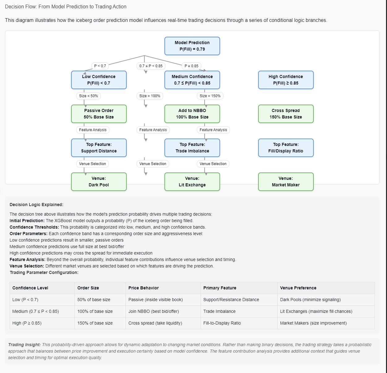
Image 3: Decision flow diagram illustrating how model predictions drive trading decisions through confidence bands and feature analysis. This probabilistic approach allows for dynamic adaptation to market conditions.
Prediction Confidence Bands
Low Confidence: P(Fill) < 0.7 - Use smaller, passive orders
Medium Confidence: 0.7 ≤ P(Fill) < 0.85 - Use full size at best bid/offer
High Confidence: P(Fill) ≥ 0.85 - May cross the spread for immediate execution
Beyond Probability: Feature Analysis
The top features driving each prediction influence venue selection and timing:
Support distance → Dark pool venues
Trade imbalance → Lit exchanges
Fill/display ratio → Market makers
This probability-driven approach allows for dynamic adaptation to changing market conditions. Rather than making binary decisions, the trading strategy takes a probabilistic approach that balances between price improvement and execution certainty.
Prediction Flow
The complete prediction flow, shown below, shows the full model architecture:
XGBoost Model Architecture
Model Configuration
The XGBoost classifier is configured with the following parameters:
| Parameter | Value | Trading Significance |
|---|---|---|
| max_depth | 4 | Moderate tree depth balances detail capture and generalization |
| learning_rate | 0.03 | Low learning rate provides more stable predictions as market conditions evolve |
| n_estimators | 250 | Sufficient number of trees to capture market relationships without overfitting |
| eval_metric | 'error@0.5' | Optimized for error rate at 0.5 threshold, balanced for trading decisions |
| min_child_weight | 8 | Controls model complexity and reduces overfitting to market noise |
| gamma | 0.2 | Minimum loss reduction required for further tree partitioning, prevents capturing random market fluctuations |
| subsample | 1.0 | Uses all training data for each tree, maximizing information capture in this case |
| colsample_bytree | 0.8 | Each tree considers 80% of features, reducing overfitting to specific market signals |
| reg_alpha | 0.2 | L1 regularization controls model sparsity, focusing on most significant market factors |
| reg_lambda | 2 | L2 regularization prevents individual features from dominating prediction, improving stability |
Tree Structure Visualization
XGBoost uses an ensemble of gradient boosted decision trees. Each tree contributes to the final prediction, with later trees focusing on correcting errors made by earlier ones.
< 6.5 ?
< 0.63 ?
< 12.5 ?
< 8.2 ?
< 0.52 ?
< 0.83 ?
< 21.5 ?
< 10.5 ?
Prediction Flow
When making a prediction for a new iceberg order, the model processes it through these steps:
Raw order data is transformed into engineered features
Features are normalized using the stored scaling parameters
The feature vector passes through all 250 decision trees
Tree 1 Output: 0.78
Tree 2 Output: 0.41
Tree 3 Output: 0.32
...
Tree 250 Output: -0.03
Tree outputs are combined and transformed to a probability
Sum of tree outputs (weighted by learning rate): 1.25
Logistic transformation: sigmoid(1.25) = 0.778
Final prediction: 77.8% probability of execution
Model Advantages for Trading Applications
| Advantage | Description | Trading Application |
|---|---|---|
| Non-Linear Relationships | Captures complex, non-linear interactions between market variables | Better models tipping points and threshold effects in market behavior |
| Robust to Feature Scaling | Tree-based models are less sensitive to feature scaling than neural networks | More stable in production when market metrics have unusual ranges |
| Handles Missing Values | XGBoost can handle missing values in features | Resilient against data quality issues in live market feeds |
| Interpretable Structure | Individual trees can be examined for trading logic | Easier to explain to regulatory bodies and trading strategy committees |
| Fast Inference | Tree traversal is computationally efficient | Low latency prediction suitable for high-frequency trading systems |
| Built-in Regularization | Prevents overfitting to market noise | More stable performance across changing market regimes |
Evaluation & Trading Strategy Implications
The evaluation metrics shown in Image 9 have several implications for trading strategy:
XGBoost Superiority: XGBoost consistently outperformed other models, especially taking into account the speed in which it is able to make a prediction and the flexibility it has regarding parameter optimization.
Feature Transferability: The dominance of order book position and imbalance features suggests that these signals may transfer well to other instruments beyond the ones tested.
Execution Time Sensitivity: The importance of “oneStateBeforeFill” features indicates that model prediction accuracy increases as the order approaches execution, suggesting a strategy that dynamically adjusts confidence thresholds based on order age.
Business Impact and Performance Metrics
The optimization trials demonstrate the model’s effectiveness, with the best XGBoost configuration achieving a score of 0.674656 on the custom evaluation metric. The trial data reveals that shorter training windows (train_size = 2) consistently perform better across all models, indicating that recent market conditions are more predictive of execution outcomes than longer historical periods.
The custom evaluation metric (max_precision_optimal_recall_score) was specifically designed to balance precision (minimizing false positives) with sufficient recall (at least 50%), making it directly relevant to trading performance where both accuracy of execution signals and capturing enough opportunities are critical.
Model Persistence & Deployment Considerations
For a production trading system, model deployment requires careful handling of model artifacts:
def save_and_upload_model(self, model, model_name):
    """
    Saves the given model to a file and uploads it to Neptune.
    """
    # Create a directory for saving models
    models_dir = "saved_models"
    os.makedirs(models_dir, exist_ok=True)

    # Save model for JVM export (compatible with trading systems)
    model_path = os.path.join(models_dir, f"xgbModel-{self.current_date}.json")
    model.save_model(model_path)
We also export the scaling parameters to ensure consistent feature transformation in production:
def write_scalers(self, model_name):
    # Extract and export scaler parameters
    scaler_params = {
        "minMaxScaler": {
            "min": self.minmax_scaler.min_.tolist(),
            "scale": self.minmax_scaler.scale_.tolist(),
            "featureNames": self.minmax_features
        },
        "standardScaler": {
            "mean": self.standard_scaler.mean_.tolist(),
            "std": self.standard_scaler.scale_.tolist(),
            "featureNames": self.non_minmax_features
        }
    }
This ensures that the model deployed to production uses identical scaling to what was used during training.
Production Integration
If implemented in a production trading system, this model would:
Extract real-time order book and trade imbalance features
Apply appropriate scaling using the persisted scaler parameters
Generate execution probability predictions
Allow trading algorithms to make more informed decisions about:
Order routing (to venues with higher fill probability)
Order sizing (increasing size when fill probability is high)
Aggressive vs. passive execution tactics
Additionally, the Neptune integration provides continuous monitoring capabilities to detect model drift in changing market conditions.
Potential Extensions
If I were to extend this project, I would:
Add market regime conditioning - adapting predictions based on volatility regimes
Incorporate order book depth information beyond level 1
Develop an adversarial model to simulate market impact of our own orders
Implement model confidence calibration to produce reliable probability estimates
Create an ensemble approach combining multiple model predictions weighted by recent performance
Conclusion: The Value of ML in Trading Systems
The complete system demonstrates how machine learning can transform trading operations by:
Extracting Hidden Patterns: The model uncovers subtle market microstructure patterns invisible to human traders
Quantifying Uncertainty: Probability-driven approaches handle the inherent uncertainty in financial markets
Adaptive Decision-Making: Dynamic parameter adjustment based on model confidence creates a more robust strategy
Continuous Improvement: Feedback loops ensure the system improves as market conditions evolve
This iceberg order prediction system represents a sophisticated approach to quantitative trading that goes beyond simple signal generation to create a complete trading ecosystem that balances predictive power with practical trading considerations.